


 MENU
MENUThe Trillion Cell Grand Challenge blog #4 by Dr. Scott Imlay, CTO, Tecplot, Inc.
Big whorls have little whorls
That feed on their velocity,
And little whorls have lesser whorls
And so on to viscosity.—Lewis F. Richardson
This is a famous quote about the nature of turbulence: the energy in turbulence cascades down to smaller and smaller eddies until, at a certain length scale, the turbulence energy can be converted by viscosity into heat. The real work, energy conversion, occurs primarily at the smallest eddy.
Breaking the Grid Into Small Pieces
Our technique for overcoming the I/O bottleneck is similar (OK, maybe the analogy is a little strained. What can I say – I like the poem!). We break the grid into small pieces called subzones, read in just the subzones we need, and perform the feature extraction on just those subzones. The technique is probably best explained with images.
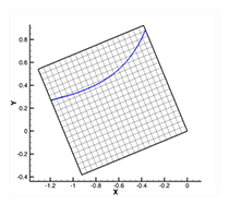
Figure 1a. Iso-contour of some variables.
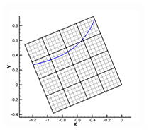
Figure 1b. Grid broken into small subzones.
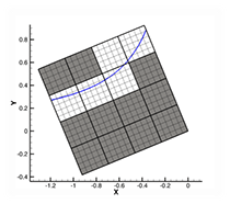
Figure 1c. Extract a fraction of the subzones.
Figure 1a shows a grid with an iso-contour line of some variables. In Figure 1b we’ve broken the grid into small subzones. If we store, in the data file or an index file, the minimum and maximum values of the iso-contour variable for each subzone, we can perform the contour line extraction without reading the shaded subzones in Figure 1c. Only 5 of the 16 subzones must be read from the file. For large 3D grids, the fraction is typically much smaller. It is not uncommon to read less than one percent of the subzones when creating a slice or an iso-surface. Furthermore, as the number of subzones goes up the number of subzones required to create a slice or an iso-surface scales with O(N^2/3), where N is the number of cells in the grid. In other words, the fraction of the subzones that must be loaded will decrease over time as the grid sizes grow.
Defeating the I/O Bottleneck
In truth, the actual algorithm is somewhat more complex. We keep the number of cells or nodes in a subzone constant (currently 256 per subzone) so the number of subzones increases linearly with the number of cells in the grid. It’s O(N). On the other hand, the number of subzones cut by a slice or an iso-surface tends to scale O(N^2/3). So a grid with 256 million cells has one million cell subzones, and roughly 10,000 of those subzones are needed to create a slice or an iso-surface. Likewise, a grid with 256 billion cells has one billion cell subzones and roughly one million of the subzones are needed to create a slice or an iso-surface. The grid is a thousand times larger and the number of subzones is only one hundred times larger. This sublinear scaling is how we defeat the I/O bottleneck.
Figure 2 shows the graph of the time to load the data from the disk and the time to transfer the data across the network. Figure 3 shows the same analysis with SZL technology and compares the total transfer times with the traditional algorithm (.plt file format) versus using SZL technology (.szplt file format).
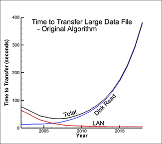
Figure 2. Time to load data from disk and transfer across network.
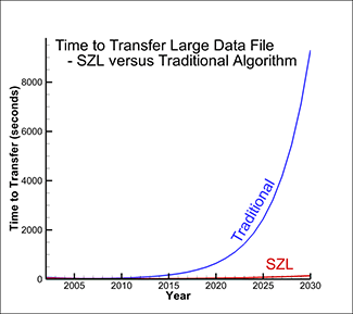
Figure 3. Time to load data with SZL technology vs. original algorithm.
As you can see, the time to load the data is still increasing slowly with time, but it is dramatically faster than the original algorithm. SZL technology makes a huge dent in the data I/O bottleneck.
Does It Work With Real Cases?
You’re probably thinking, how well does it work with real cases? The following plot shows the performance for five datasets of various sizes. The smallest case is roughly a million cells and the largest is two billion cells. All but the largest case are real CFD solutions. All of the cases are faster than “Tecplot 360 2013” and all but the smallest case are at least ten times faster. The largest case is roughly 120 times faster with the latest Tecplot 360 and SZL than it was with “Tecplot 360 2013”. These are very dramatic results – SZL clearly works!
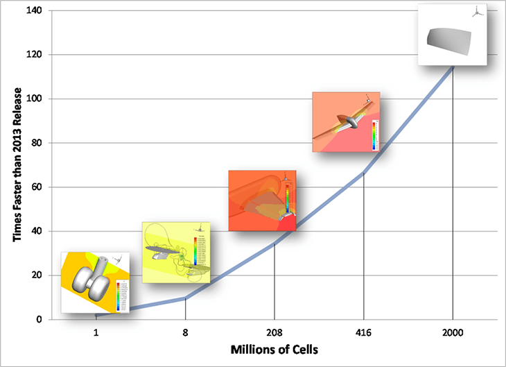
These are very dramatic results – SZL clearly works!
Blogs in the Trillion Cell Grand Challenge Series
Blog #1 The Trillion Cell Grand Challenge
Blog #2 Why One Trillion Cells?
Blog #3 What Obstacles Stand Between Us and One Trillion Cells?
Blog #4 Intelligently Defeating the I/O Bottleneck
Blog #5 Scaling to 300 Billion Cells – Results To Date
Blog #6 SZL Data Analysis—Making It Scale Sub-linearly
Blog #7 Serendipitous Side Effect of SZL Technology