


 MENU
MENUWhich came first, the chicken or the egg?—Aristotle
In developing the technology to meet the Trillion Cell Challenge we struggled with the visualization version of this classic causality dilemma, and I finally have an answer! But first, a little background.
Subzone Load-on-Demand (SZL) Technology
As many of you know, Tecplot 360 utilizes a new technology—called SZL (Subzone Load-on-Demand)—that minimizes the amount of data loaded by Tecplot 360. The basic idea is to divide a large dataset into small pieces, or subzones, and load only those subzones needed for the desired plot.
For example, to make an isosurface of pressure for a large dataset, like the NASA trapezoidal wing shown in figure 1, only the subzones with a pressure range (pmin, pmax) that contain the desired isosurface value of pressure will be loaded.
Tecplot 360 is Orders of Magnitude Faster
To generate the isosurface shown in figure 2, only 1.5% of the subzones need to be loaded. This makes isosurface generation in the new version of Tecplot 360, Tecplot 360, orders of magnitude faster than previous versions (and faster than competitor codes) that load pressure, for the majority of the data points in the dataset.
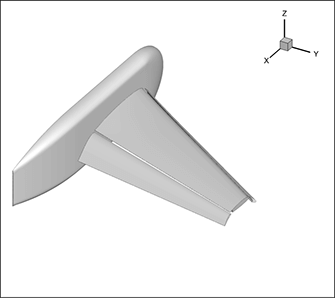
Figure 1. NASA Trapezoidal Wing (High-Lift Prediction Workshop) Geometry.
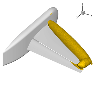
Figure 2. Pressure isosurface for NASA Trapezoidal Wing (High-Lift Prediction Workshop).
The Chicken or the Egg?
But, you ask, what if pressure isn’t stored in the dataset? What if only the conservative variables (ρ, ρν, ρυ, ρω, Ε) are stored? This is a common scenario in PLOT3D format files generated by codes like Overflow. This is the classic “chicken or the egg” scenario. Ranges of pressure for each subzone (the egg) determine which subzones to load, but pressure (the chicken) doesn’t exist in the file.
For ideal gases, pressure can be computed from the conservative variables using the following formula:

One solution would be to load all five conservative variables, compute pressure at every point in the dataset, compute the pressure ranges, and proceed as before. Unfortunately, this would end up loading all the data—violating the SZL goal to minimize the amount of data loaded.
It’s the chicken or the egg; the “Kobayashi Maru”; the no-win situation. Or is it?
It turns out that interval arithmetic can be used to compute bounds for the range of the pressure in each subzone without actually computing the pressure in the subzones. Interval arithmetic allows you to estimate the range (actually bounds of the range) of the computed variable from the ranges of the input variables and the equation to be computed. With SZL, interval arithmetic is used to determine which subzones to load and only the new variable in the loaded subzones is computed. However, because interval arithmetic will overestimate the ranges of the computed variable for each subzone, it is possible that many unneeded subzones will also be loaded.
Testing the Impact of Subzone Load-on-Demand (SZL)
We used the NASA Trapezoidal Wing case (figure 1) to test the impact of this approximation when computing, on demand, the pressure from the conservative variables. We also pre-computed a new pressure variable so that we could compare the number of subzones loaded.
The Trapezoidal Wing dataset contains a total of 800,606 cell subzones. Using the pre-computed pressure directly, subzone load-on-demand loads 11,905 subzones (1.49% of the total). Using interval arithmetic with the ranges of (ρ, ρυ, ρu, ρω, Ε), Subzone Load-on-Demand will load 13,349 subzones (1.67% of the total). That is only 12% more subzones than were loaded with the pre-computed pressure.
So, you don’t need the chicken, the egg can come first!
In the next blog, I’ll discuss how Subzone Load-on-Demand (SZL) allows significant compression of finite-element node maps, leading to smaller data files.
Blogs in the Trillion Cell Grand Challenge Series
Blog #1 The Trillion Cell Grand Challenge
Blog #2 Why One Trillion Cells?
Blog #3 What Obstacles Stand Between Us and One Trillion Cells?
Blog #4 Intelligently Defeating the I/O Bottleneck
Blog #5 Scaling to 300 Billion Cells – Results To Date
Blog #6 SZL Data Analysis—Making It Scale Sub-linearly
Blog #7 Serendipitous Side Effect of SZL Technology