


 MENU
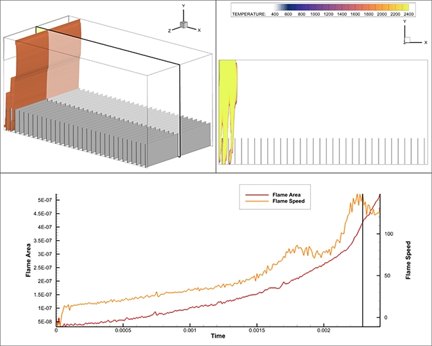
MENUEngineers from Convergent Science are studying the effect of obstacles on the time taken for deflagration to detonation transition (DDT) in various configurations (blockage ratio and stagger ratio). Ideally one would like to delay DDT. This study could help understand how blockages can be used to control DDT.
Deflagration describes combustion at a velocity slower than the speed of sound. You see deflagration typically as common flame in everyday life, like in a fireplace or on burning candle. Detonation describes combustion at a higher velocity than the speed of sound. You see this in explosions that release shockwaves, such as a fighter jet breaking the sound barrier or a gas leak in a mine or a factory.
To quantify the results of the simulations, they wanted to compute the flame area (represented by an isosurface at 1800 degrees) and the flame speed (determined by the max x-position over time, dXmax/dt). Measuring flame area gives information on flame wrinkling which they wanted to correlate with flame speed. They also wanted to see how flame wrinkling changes as flame transitions from deflagration to detonation.
This guide explains the techniques and features used in Tecplot 360 and PyTecplot to extract this information from the simulation results.
Data and scripts for this case can be downloaded here: FlameFrontAnalysis.tar. To run the scripts, be sure to unpack Data.tar.gz to a sub-directory called Data first.
Computing the flame area and flame speed using Tecplot 360 and PyTecplot
Computing Flame Area and Flame Speed Using Tecplot 360 and PyTecplot
The two quantities we need to compute from this dataset are flame area and flame speed. First, we need to define the flame front. Once we have the flame front defined, we can compute the flame area and flame speed.
Computing Flame Area
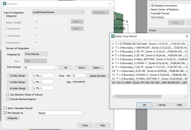
Flame area is relatively simple – you can use Analyze > Perform Integration > Length/Area/Volume to compute the area of the isosurface. Recall that Tecplot 360 performs calculations on Zones – so we must first extract the isosurface to zones before we can use the integration feature. So, the rough steps are:
- Define an isosurface at temperature = 1800, which defines the flame front
- Data > Extract > Iso-Surfaces Over Time
- Analyze > Perform Integration
- Choose Length/Area/Volume
- Integrate by Time Strands and select the strand associated with the isosurface you extracted.
- Check the Plot Results As toggle
- Press Integrate
Computing Flame Area
At this point you will have a new frame with a line plot that represents the flame area. Select this frame and save this data to a data file using File > Write Data…
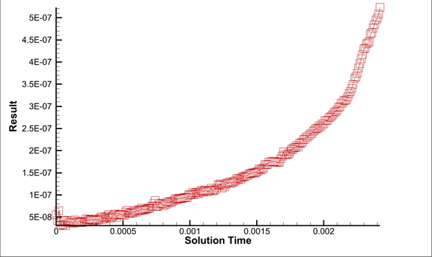
Flame Area
Computing Flame Speed
The flame speed is defined as dXmax/dt. Tecplot 360 cannot compute this equation with its built-in equation processing, so we’ll use the PyTecplot scripting language to not only extract the maximum X-position from the flame front at each timestep, but also compute the flame speed. Once we’ve computed the results, we’ll save the results to a Tecplot ASCII file.
The PyTecplot script below will connect to a live, running instance of Tecplot 360 to extract the information. There are a couple prerequisites to running this script:
- Ensure you have Python 3 and PyTecplot installed
- Save the script (below) to a file (for example, compute_flame_speed.py)
- Enable PyTecplot connections via Scripting > PyTecplot Connections…
- Ensure that the frame with the CONVERGE data is the active frame. As you can see, the script below queries for the dataset associated with the active frame.
Once you’ve satisfied the pre-requisites, simply run the script:
> python -O compute_flame_speed.py
Python Script
import tecplot as tp
tp.session.connect()
ds = tp.active_frame().dataset
iso_zones = ds.zones("Iso*")
times = []
maxx = []
speed = []
# Assuming that the zones are given in time order
for z in iso_zones:
maxx.append(z.values("X").max())
times.append(z.solution_time)
if len(maxx) == 1:
speed.append(0)
else:
dx = (maxx[-1] - maxx[-2])
dt = (times[-1] - times[-2])
speed.append(dx/dt)
# Save the results to a Tecplot data file. We do this by creating a
# new dataset in Tecplot 360 with the results and saving to a file.
new_frame = tp.active_page().add_frame()
ds = new_frame.create_dataset("Flame Speed", var_names=["Solution Time", "Flame Speed"])
zone = ds.add_ordered_zone("Flame Speed", shape=len(times))
zone.values("Solution Time")[:] = times
zone.values("Flame Speed")[:] = speed
tp.data.save_tecplot_ascii("flame_speed.dat", frame=new_frame)
# We’ve saved the data to disk and no longer need the frame around
tp.active_page().delete_frame(new_frame)
Plotting the Results
We now have one data file with the flame area results and another file with the flame speed results. To plot the results, simply create a new frame in Tecplot 360, then load the two files together.
By default, Tecplot 360 plots only the results for the first zone, so you’ll have to use the Mapping Style dialog to plot the data of interest. As seen in the image below, we’ve created two separate line maps, each plotting different data. Because flame area and flame speed have very different magnitude, we’re using the Y2 axis to plot the flame speed.
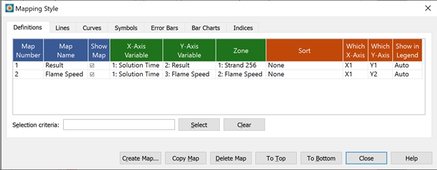
Mapping Style dialog in Tecplot 360
To create the final plotted result, we’ve added a line legend and modified the first line map name from “Result” to “Flame Area.” We’ve also renamed the Y1 axis title to use “Flame Area.”
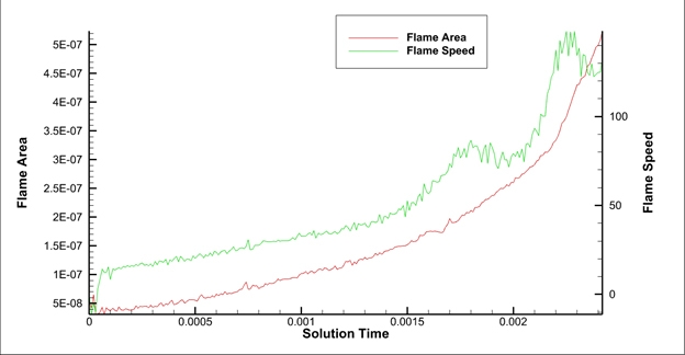
Final plotted result in Tecplot 360
Summary
In this how-to guide you learned the following:
- Loading CONVERGE data.
- Defining and extracting an isosurface.
- Use of Length/Area/Volume integration.
- Use of PyTecplot to extract data and to create new results.
- Plotting of resulting data.
Appendix – Automating the Entire Process
Note that this entire process can be fully automated using PyTecplot, so that the resulting data and plots can be created by running a single script. See the FlameFrontAnalysis.py script in the downloadable package FlameFrontAnalysis.tar, which shows how we automated the entire process. The script uses a slightly different method to collect the flame area – rather than having Perform Integration create a new plot, this script uses Perform Integration to compute and collect the flame area at each timestep. In the end this script saves the flame area and flame speed results to a file and creates a Tecplot 360 layout file for viewing the results.