


 MENU
MENUThe purpose of this article is to help you understand when you should use Parallel FieldView and its unique Auto Partitioner capability.
Parallel CFD Post-Processing with FieldView – Basic Principles
To accelerate the processing of your simulation results, FieldView uses two forms of parallelization in combination:
- Multi-threading, which uses multiple threads within a process, executing concurrently and sharing resources. This is used automatically by FieldView when computing streamlines, new variables, etc.
- The Message Passing Interface (MPI), which is a communication protocol designed to function on parallel computing architectures.
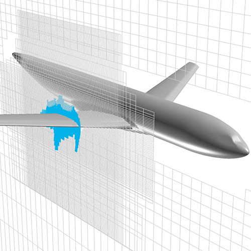
Example of a structured overset multi-grid topology
For today, we’ll focus on the latter.
MPI Parallel can be described as a “divide and conquer” approach. Work gets shared between FieldView processes based on blocks of cells (called “grids” in FieldView) as defined in your mesh file. There are many reasons for a CFD domain to be divided into grids. To name a few:
- To represent different materials (fluid, solid, porous)
- To locally control mesh refinement and cells quality
- To “wrap” bodies with boundary layer aligned cells
- To automatically refine the mesh
- Or, your CFD solver running in MPI Parallel may have saved its mesh partitions as grids
Except for the latter case, none of the reasons above will lead to cells being distributed evenly across grids.
The Problem – Uneven number of cells per grid
With cells not being evenly distributed across grids, FieldView may or may not be able to balance the workload across processes. Note that this problem is not specific to FieldView: all CFD post-processors capable of MPI Parallel rely on the same principle.
The most extreme example would be a mesh file with a single grid. MPI Parallel is unable to help in such a case as one process only will have to do all the work while other processes remain idle.
With a larger number of grids, FieldView will be capable of balancing the work across processes in a lot of cases. In the figure below, let’s look at the real-life scenario of a 17 grids mesh consisting of 5 grids encompassing the majority of cells, and 12 smaller grids. The plot on the right represents how FieldView will assign grids to 8 processes to achieve good load balancing.
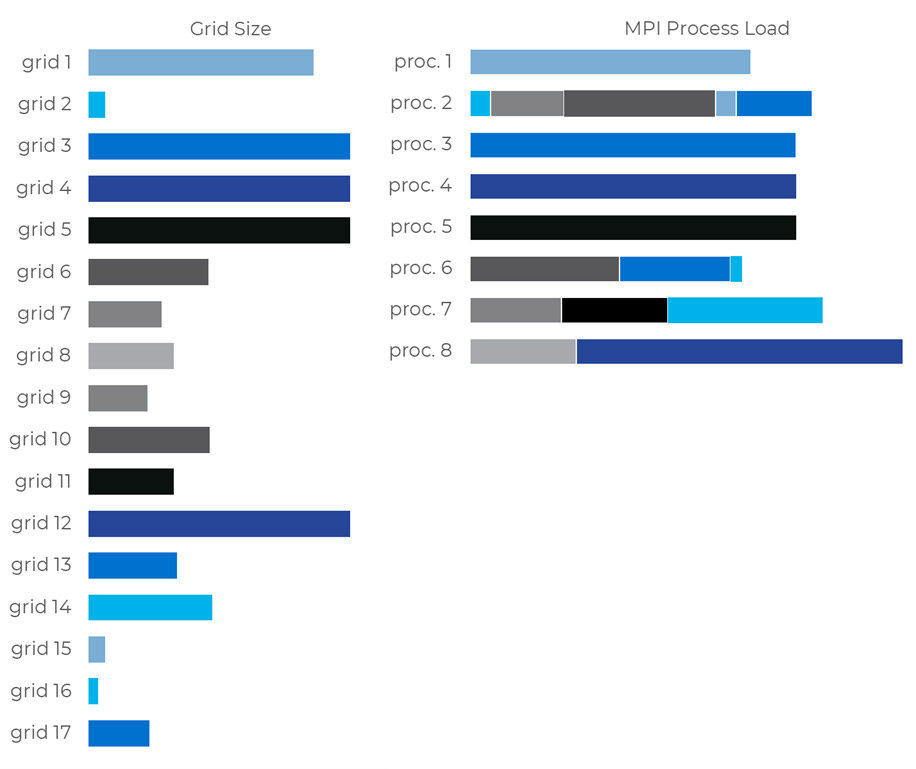
Figure 1. A 17 grids mesh processed with FieldView Parallel running on 8 processes, leading to good load balancing.
But as you try to gain more performance or access more distributed memory by running more processes, obtaining good load balancing may just become an impossible task. In the figure below, we’re looking at the same case now running 16 processes.
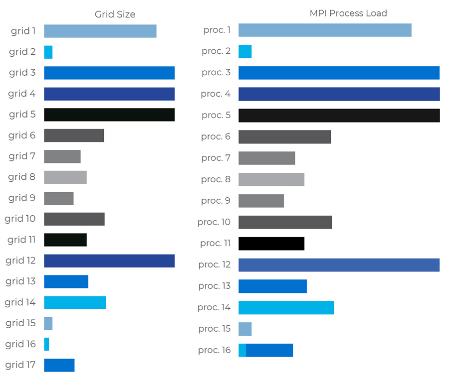
Figure 2. A 17 grids mesh processed with FieldView Parallel running on 16 processes, leading to poor load balancing.
In conclusion, for such a mesh file, there would be little to no benefit to increasing the number of processes beyond 8.
No benefit, until now…
The Solution – FieldView’s Auto Partitioner
With the introduction of FieldView’s unique Auto Partitioner, you can now take advantage of FieldView’s MPI parallelization at higher process counts than would have made sense for your meshes in the past.
Simply activate the Auto Partition option (as show in figure 3) and FieldView will automatically partition your largest grids on-the-fly, during the Data Input process, to obtain a new set of partitions optimized for the number of processes you’re running. If no new partition is needed, your mesh will just be imported without extra processing.
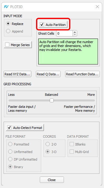
Figure 3: location of the Auto Partition option on the PLOT3D Data Input panel
Note that for this option to be enabled, you will need to be reading PLOT3D or OVERFLOW data in parallel (we’re planning on adding support for more readers in the future), with either a FieldView Parallel 32 or 64 license.
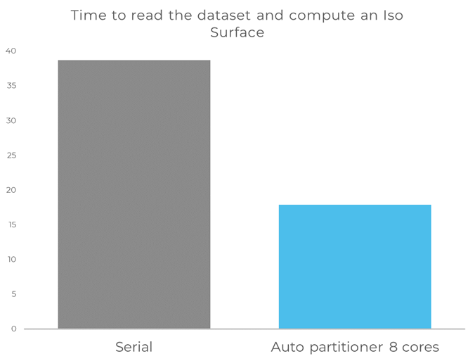
Going back to the extreme example of single grid mesh (here in PLOT3D format with 200 million cells), the speedup is over 2x on 8 processes for reading the dataset, computing an Iso Surface and rendering it.
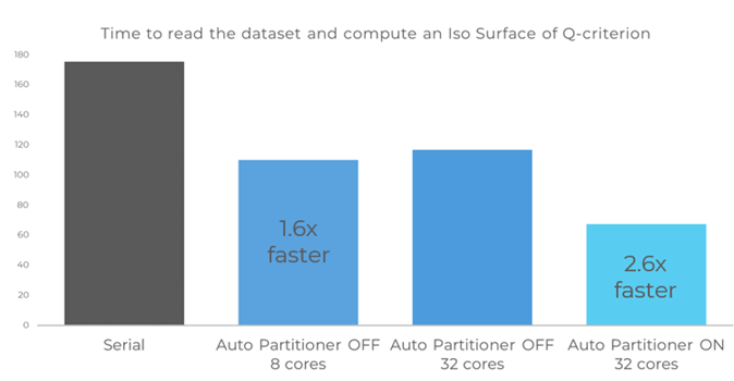
For the real-life case also mentioned above of 17 grids (PLOT3D format with over 400 million nodes), the Auto Partitioner allows additional speedups beyond 8 processes.
Limitations
MPI Parallel can’t accelerate all operations in your post-processing workflow. The rendering of your scene, for instance, is mostly handled by the GPU. So, it won’t be affected by the number of processes running on the CPU. Moreover, although the creation of most objects in FieldView has been parallelized for MPI, the speedup depends on the number of processes that will be contributing to its computation and hence the number of grids it is traversing. The figure below shows what operations typically benefit the most/less from MPI Parallel.
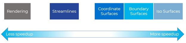
Depending on what operation dominates your post-processing workflow, you should expect a different speedup overall. Typically, the more time is spent on reading data and computing large surfaces, the more benefit you’ll experience.
How can I time these speedups myself?
It is quite easy to monitor the run time of an automated FieldView job being run under different configurations.
The first thing you need is an FVX script that will have instructions to be executed automatically by FieldView. As an example, we’ll look at an FVX script that reads a case, loads a Formula Restart to define a new variable for Q-criterion, then creates an Iso Surface based on this variable.
The first function call will read your mesh and results. For a binary PLOT3D case with grid and Q files, it looks like this:
read_dataset( {
   data_format = "plot3d",
   server_config = "Local licensed parallel",
   input_parameters = {
      xyz_file = {
         name = "/file_path/my_grid.x ",
         options = {
            format = "binary",
            coords = "3d",
            multi_grid = "on",
            iblanks = "on",
            auto_partition  = "on",
        }
      },
      q_file = {
         name = "/file_path/my_results.q ",
         options = {
            format = "binary",
           coords = "3d",
           multi_grid = "on",
           iblanks = "on",
         }
      },
   }
} )
Next, we’ll load the Formula Restart
fv_script("RESTART FORMULA /file_path/restart.frm")
For a PLOT3D Q file, the Formula Restart file only needs to contain these 3 lines
formula_restart_version: 1
Q-criterion
Qcriterion("Velocity Vectors [PLOT3D]")
Finally, the last function call will create an Iso Surface based on this new variable.
create_iso(
   {
      iso_value = { current = 10},
      display_type = "smooth_shading",
      iso_func = "Q-criterion",
   }
)
FieldView has a super useful command called TIMING ON/OFF for timing any operation. The result will be printed to console.
Putting it all together, here is the full FVX. Open the FVX file.
fv_script("TIMING ON")

read_dataset( {
   data_format = "plot3d",
   server_config = "Local licensed parallel",
   input_parameters = {
      xyz_file = {
         name = "/file_path/my_grid.x",
         options = {
            format = "binary",
            coords = "3d",
            multi_grid = "on",
            iblanks = "on",
            auto_partition  = "on",
         }
      },
      q_file = {
         name = "/file_path/my_results.q",
         options = {
            format = "binary",
           coords = "3d",
           multi_grid = "on",
           iblanks = "on",
         }
      },
   }
} )

fv_script("RESTART FORMULA /file_path/restart.frm")

create_iso(
   {
      iso_value = { current = 10},
      display_type = "smooth_shading",
      iso_func = "Q-criterion",
   }
)

fv_script("TIMING OFF Time to read my case and create and Iso")
The next thing you need to know is how to execute this script automatically. This is done by launching FieldView with the command line below:
fv -fvx my_script.fvx -batch
Use the “-batch” option if you want FieldView to run “headless”.
Say you want to compare the following runs:
- Serial
- Parallel with 8 processes
- Parallel with 32 processes, Auto Partitioner OFF
- Parallel with 32 processes, Auto Partitioner ON
The table below shows the adjustments you need to make to your FVX, in addition to editing file paths and names:
| Serial | Remove the “server_config” line |
|---|---|
| Parallel with 8 processes | Keep the “server_config” line Run with a standard FieldView license on a system with at least 8 cores |
| Parallel with 32 processes, Auto Partitioner OFF | Keep the “server_config” line
Run with a FieldView Parallel 32 license on a system with at least 32 cores auto_partition = “off”, |
| Parallel with 32 processes, Auto Partitioner ON | Keep the “server_config” line
Run with a FieldView Parallel 32 license on a system with at least 32 cores auto_partition = “on”, |
If your system has less than 32 cores, FieldView will adjust the number of MPI processes automatically.
Be aware that if you’re reading the same file several times in a row, most operating systems and file systems are configured to automatically cache that file. This will make subsequent reads faster. For a fair comparison, the cache should be flushed between reads. If you don’t have the credentials to flush the cache, you can also change the mesh and result files you read at each run, for instance by picking another time step of the same simulation. This will force a true read for each run.
If you need help performing these operations, please don’t hesitate to contact us at support@tecplot.com. We would love to hear about your own benchmark results.
Future Work
Our Development Team is already working on improvements to our Auto Partitioner.
In FieldView 21, when the Auto Partitioner flags grids that are too large for good load balancing, these grids get actually split, leading to the creation of new grids. This has an impact on many areas of FieldView: grid numbers, IJK dimensions for each grid, etc. The first improvement will be to make the Auto Partitioner’s effect totally transparent to the user: the mesh will appear as it is on file, with the new partitioning only existing under the hood.
Going forward, we’ll also work on extending this feature to more Data Input options.
If you’d like to try the Auto Partitioner but don’t have access to a FieldView Parallel 32 license, feel free to contact us for a free evaluation.
Also watch this quick overview video of the FieldView Auto Partitioner.