Shadowgraph Technique in Tecplot 360

Description

This is a quick tutorial on using Tecplot 360 to look at pressure and density gradients. I’ve had several people ask me questions recently about Schlieren diagrams or Schlieren images using Tecplot 360.

Schlieren is an optical technique looking for inhomogeneous density gradients in, typically, translucent media like air. This works really well when you are analyzing supersonic flow because there are large changes in the density as the object passes through shockwaves. And these density changes, you can actually see in an image. In computational methods, you can use the shadowgraph technique to look at these same pressure gradients.

In Tecplot 360, I have loaded a supersonic airfoil. We are looking at one slice of that airfoil. The first thing we want to do is to calculate a variable. The variable we’re going to calculate is shadowgraph.

Calculating Shadowgraph

1. Choose Calculate Variable… from the Analyze menu
2. Click Select… and choose Shadowgraph from the list of variables.
3. It is a relatively small data set, so uncheck Calculate on Demand.
4. Click Calculate.
5. In this case, we have field variables that have not been specified, so we will need to define our State Variables.
   1. Choose Field Variables… from the Analyze menu
   2. For pressure, select Pressure and click Select… and choose Pressure from the list.
   3. For density, choose Density, and click Select… and choose Rho from the list.
   4. Choose the Convective Variables U and V and click OK.
   5. Click Calculate. Click OK to close the windows.

The calculations are now complete.

Displaying Shadowgraph

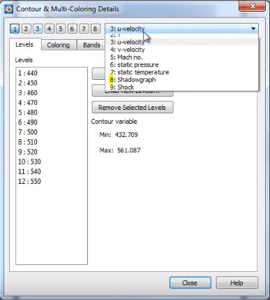
Now open the Contour Details… dialog and choose Shadowgraph to the right of the number buttons.

Turn on contour for shadowgraph, but you will not yet see what you’re looking for.

In the Contour Details… dialog Coloring tab, use the GreyScale colormap. And now you can see the shadowgraph in more detail.

Another way to do this is using a continuous spectrum. However, the small variations get washed out if you move to continuous coloring. The banded coloring is an easier way to see the gradients. You can also use the add and subtract contour icons to try to put a little more detail on the fine structure.

But there you have it. A simple way to calculate shadowgraph function to create the equivalent of a Schlieren diagram.

Thanks for watching!

Related Videos