


 MENU
MENUThis Case Study was contributed by Dipl.-Ing. Paul Kamrath, Research Engineer, Institute of Hydraulic Engineering and Water Resources Management, Aachen University, Aachen, Germany
The Engineer
Paul Kamrath is a research engineer at the Institute of Hydraulic Engineering and Water Resources Management (IWW), part of Germany’s Aachen University (RWTH Aachen). Over twenty full-time researchers and fifty student researchers work at IWW.
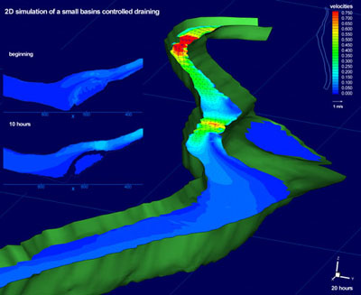
Figure 1. Using Tecplot 360, Paul Kamrath visualizes a reservoir draining over time. His model estimates the risk of stored toxic sediments mobilizing, reducing downstream water quality.
IWW consists of five groups:
- Hydraulics and numerical methods for river flow calculations
- Groundwater modeling
- Risk assessment for dams and hydraulic structure safety
- Sediment transport processes and water quality simulation for rivers
- Automatic optimization methods
Paul develops numerical methods for river flows and free-surface flow hydraulics. In addition, he works on methods to determine resistance parameters in rivers and channels.
His research is funded by government, river and environmental associations, energy supply corporations, as well as the German Research Foundation.
The Simulation
Reservoirs and lakes have significant influence on water quality. Water stays in these systems for several months — even years, causing heavy metals, toxic substances and other fine river sediments to settle at the bottom. This settling creates better water quality downstream.
Flood events produce higher flow velocities, increasing shear stress on the reservoir bottom. Shear stresses can erode decades of sediment build-up and dramatically reduce downstream water quality.
This phenomenon makes predicting the influence of sedimentation and erosion on water quality very important. In response, IWW developed a numerical River Simulation Model (RISMO) to calculate velocities and shear stresses at lake and reservoir bottoms.
Using a finite-element method, RISMO solves shallow water equations obtained by vertical integration of the Navier-Stokes equations, as well as the continuity equation. A wet-dry algorithm considers overflow and dry regions. A decoupled transport module calculates transport rates when flow calculations are completed.
The Plot
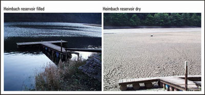
Figure 2. Views of the Heimbach reservoir.
The Heimbach reservoir is located approximately 50 kilometers from the city of Aachen, Germany. Originally built in 1935, it is the smallest of a number of reservoirs storing drinking water.
Approximately 2000 meters by 150 meters, with water depths between 1.5 meters and 6 meters, the reservoir is more like a river than a lake. Its main purpose is to balance widely varying outflow from power plants, maintaining adequate water levels downstream.
In the late 1990s a plan was developed to repair the reservoir’s damaged concrete dam. The basin was emptied in 2001 during restoration work.
To estimate the risk of stored sediments mobilizing during the drainage, Paul performed two-dimensional RISMO simulations. (Since the basin’s depth is small compared to its width, a 2-D model is sufficient.) He calibrated his model with Acoustic Doppler Current Profile (ADCP) measurements taken during drainage. His results also help validate theories about cohesive sediment erosion capabilities developed at the IWW.
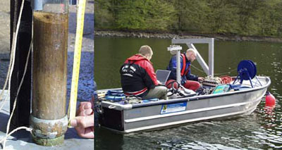
Figure 3. Sediment probe (left) and ADCP measurements (right).
RISMO results are imported directly into Tecplot 360 using an AVS-UCD data loader built with Tecplot ADK. The main image displays a three-dimensional view of the reservoir illustrating drainage at different times. The image in Figure 1 was created by:
- Scaling the basin depth by a factor of 10 (since the range is small)
- Projecting the 2-D data to the water surface. This is performed by using Tecplot 360’s Data Alter (Z-value equal to the water surface)
- Excluding dry regions with Data Blanking (If flow depth H is less than or equal to .02 at any corner, blank entire cell)
- Linking remaining frames using 2D plotting
- Adding a small frame next to the contour legend with a rotated view of the boundary
Tecplot 360
Paul started using Tecplot 360 five years ago. Prior to Tecplot 360 he used AVS — he switched because he felt Tecplot 360 was more intuitive, making visualization easier.
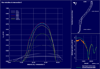
Figure 4. Flow velocities at a cross section.
Paul’s typical Tecplot 360 usage includes:
- Creating contour plots for general overviews of his simulation
- Generating XY plots for precise information at cross-sections
- Building animations for unsteady cases (Animations are great for presenting his results to audiences)
- Placing streamtraces for visualizing large eddies
For Paul, Tecplot 360’s three greatest strengths are:
- Viewing results on-the-fly
- Quality print output
- User-defined, custom post-processing routines
Paul’s Tecplot 360 tips:
- Use Tecplot 360 for any data that needs to be plotted. Whether your data is measured or simulated, it only needs to be formatted as ASCII-text to import
- Use Copy Style to File to create large numbers of similar plots in a short time
- Create a set of standard styles so you can plot your data in seconds