


 MENU
MENUContributed by Paul D. Orkwis, PhD & John Ratzlaff, University of Cincinnati
Graduate students along with their professors at the University of Cincinnati’s Department of Aerospace Engineering-Gas Turbine Simulation Laboratory use advanced software tools to study the physics of airflow and how it impacts the performance of aircraft engines. They share the results of their research with academia, industry and government laboratories.
The Researchers
Paul D. Orkwis, PhD, Director of Graduate Studies, at the University of Cincinnati’s Department of Aerospace Engineering, along with research assistant and graduate student, John Ratzlaff, studied how cooling holes operate and the flow physics of cooling holes on a prototype of an engine blade.
Paul D. Orkwis, PhD, is Director of Graduate Studies at the University of Cincinnati’s Department of Aerospace Engineering. His research assistant and graduate student is John Ratzlaff. Together they studied how cooling holes operate and the flow physics of cooling holes on a prototype of an engine blade.
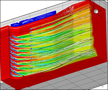
Figure 1: Temperature on the surface on an unloaded, cooled blade, along with streamlines of the main flow and the coolant.
To understand the flow physics of cooling holes, Orkwis and Ratzlaff used CFD++ software from Metacomp Technologies to perform a CFD analysis on a CAD model of a simplified engine blade that was tested experimentally in the UC Combustion Research Laboratory. After creating the CAD model of the blade, they generated a grid of the flow field inside the geometry. Next, using CFD++, they simulated the flow of the coolant and the main flow.
“We didn’t just do the flow over the surface, we did the flow through the holes and inside the tube that feeds the flow, which is called the plenum,” says Orkwis. “In this case it’s a lower-temperature fluid that comes out of the holes compared to a higher-temperature main flow.”
Plotting Results in Tecplot 360
Upon completion of the analysis, the results were plotted in Tecplot 360 software. The resulting plot (Figure 1) shows the temperature on the surface on an unloaded, cooled blade. The blade is shown with streamlines of the main flow and the coolant.
On the plot, the white streamlines represent the coolant, while the black streamlines represent the higher-temperature main flow. “The flow was seeded inside the feed chamber and allowed to exit the holes and follow the cool gas that’s coming out,” says Orkwis. “The dark or black streamlines are seeded upstream and the plot shows how that hot fluid mixes with the cool fluid.”
“I would say that Tecplot 360’s three greatest strengths are: good functionality in terms of streamlines and contours, ease of use with data formats, and ability to batch process.” – Paul Orkwis, University of Cincinnati
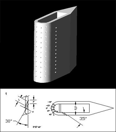
Figure 2: The blade design consisted of a thickness of 0.9″, a span of 3″, and a chord of 4″. Holes were located at 15° (s/d = 1.9) and 40° (s/d = 5); Angled Downward at 60°, 3rd Row at s/d = 20.9; Angled at 35° off blade wall. Hole Dimensions: D/d = 14.4, L/d = 5.1, P/d = 4
Tecplot 360 Reveals Unseen Flow Physics
The Tecplot 360 visualization revealed some unexpected results. The plot showed how the cooling film bathed the surface with cool flow and mixed with the hot main flow and other coolant jets. It also showed the coalescing of jets as demonstrated by the exit plane contour. Dr. Orkwis explained why the span-averaged temperature plots are not smooth.
“If you increase the amount of coolant you’ll get hot spots on the surface because the coolant doesn’t just lay flat on the surface. It shoots out into the stream and you lose its usefulness.” – Paul Orkwis, University of Cincinnati
The researchers also examined the results of their CFD analysis by creating a plot showing the temperature profiles. These profiles represent the average temperature at the exit, which is not smooth, but jagged. “You see some of that behavior ‘when you look at the back wall. We have contours there and you can see that the coolant looks like a series of waterfalls along the back wall where the flow is going out,” says Orkwis. “That’s an indication of the jets pairing together. They coalesce. They stay together, which means that some areas will get really cool, but others won’t. That’s not a good design.”
Fully Understanding the Aerodynamics
Dr. Orkwis explains why it is so crucial to fully understand—through the use of advanced CFD and visualization tools—the aerodynamics of the component. “The aerodynamics of it is a big part because you need to know where that coolant is going,” Orkwis says, “It’s not just a question of knowing how hot is the surface but where is the hot flow coming from. And why are the jets doing what they’re doing.”
After viewing the plot, Orkwis and Ratzlaff decided to do another run. This time they increased the amount of coolant to see how that would affect the fluid dynamics of the design. “Bad things happened for the cooling properties because the cooling jets detach from the surface,” says Orkwis. “If you increase the amount of coolant you’ll get hot spots on the surface because the coolant doesn’t just lay flat on the surface. It shoots out into the stream and you lose its usefulness.”
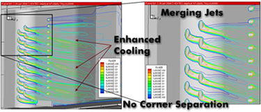
Figure 3: Blowing film effectiveness. The plots show that with merging jets and enhanced cooling, no separations exist.
Sharing Plots Help Other Students Learn
Student researchers use the plots created with Tecplot 360 software to share the results of their research with industry, academia, and government research labs. In addition, the plots are also shared with larger student research groups so each student benefits from knowledge obtained through the work of other students.