Compare CFD vs Measured Data through Extractions

Today I will show you how to get more out of your simulation data by using data extractions. Many of you know Tecplot 360 can show you your simulated data in vibrant 3D views. But we also know that many engineers make decisions by looking at single values or line plots. And that is where data extractions come in.

I am Scott Fowler, the product manager of Tecplot 360. I have been with Tecplot since 1999. One of my favorite things about this job is being able to interact with such an intelligent people like yourselves. Thank you for making my job so interesting!

Four Methods for Extracting Line Data in Tecplot 360

Video Timestamp – 0:02:06

I am going to show you four techniques for extracting line data. You can use the first three techniques directly through the Tecplot 360 user interface. The fourth uses a new function in PyTecplot, our Tecplot 360 Python API (application programming interface).

1. Extract from Polyline
2. Extract precise line
3. Extract a slice from a slice
4. Probe on Surface – PyTecplot only

Demo, Data and Scripts

Video Timestamp – 0:03:45

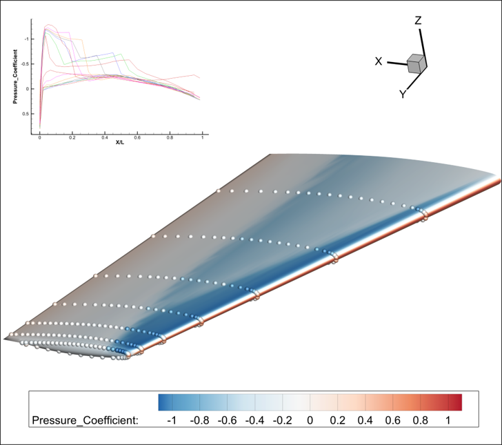
The data, layout and scripts used in this demonstration are available for download. I am using the ONERA M6 Wing data simulated using SU2. In Figure 1, the spheres you see represent the locations of the measured data on the wing. The experimental data has been normalized and is also in the examples folder.

Download the Data, Script, and Layout Files

Method 1: Extracting from Polyline

Video Timestamp – 0:05:04

First, I will look at a way of extracting data using “Extract from Polyline.” This is a helpful tool for getting a quick and dirty view of what is happening on the surface. I am going to turn off the scatter layer, so we see just the wing.

1. Select the Polyline tool and click two points along the leading edge of the wing. Now I have clicked once, clicked twice, and now it is just kind of hanging here. Right-click to finish drawing the Polyline.
2. Select the Polyline by clicking on it, right-click on the line select Extract points which brings up the Extract Data Points dialog. This dialog gives me the choice of how many points along the line to extract. I can extract an even distribution of points along the line. The default is 200 spaced evenly along that line. (Or I can extract the points that define the geometry. I defined the Polyline by only two points, one at the start and one at the end, so I don’t want this option). I want data in the middle, evenly spaced, so I am going to select regular points along that geometry.
3. Click Extract and the extraction is now complete. Open the Data>Data Set Information dialog. You can see that I have a zone called Extracted Points with 200, and it has all of the variable values associated with it.
4. Plot these results using the Create New Frame tool . Click and drag to create a new frame.
5. Change the Plot type to XY line. The new frame will inherit the data that was in the original frame. For the X-Axis, select y. For Y-Axis, select Pressure_Coefficient. For Zone, select the Extracted Points.

This is an easy way to get a quick line-plot view of your data using the Extract from Polyline tool.

Just a couple of notes about the Extract from Polyline tool. You can do arbitrary Polylines. Or click a number of points and extract a Polyline from these points. You may want to do this if you are in geoscience and you want to extract points on the surface of the ocean, or up an inlet or river. A tool like this is useful to follow the path of that river. And if you have transient data, when you have the Polyline selected, you can go to data, and extract the geometry over time.

One warning about Extracting from Polyline. Orientation of my data matters. I will turn off the mesh so you will see only the Polyline. If I rotate my plot, I am going to get a different set of points. Tecplot 360 extracts these points by shooting a ray from your eye through the screen, through the monitor, through that point, and then hitting the surface. Now I am going to get a point right on this line, but if I rotate my plot slightly, I am going to get a line in a very different location. This is important to know when you are writing scripts. If you are running Tecplot 360 in batch mode, you need to make sure that you do not change the orientation of your plot; that it stays the same relative to your Polyline.

Method 2: Extracting a Precise Line

Video Timestamp – 0:09:00

To specify an exact XYZ starting location and ending location, use the Extract a Precise Line (Data>Extract Precise Line). This tool is ideal for extracting data from a volume because we are specifying exact XYZ locations. Extracting from a surface like this, has similar issues to extracting the Polyline geometry in that it is dependent on the orientation the plot.

To look at a line that goes from the leading edge to the trailing edge, use the probe tool .

Click on the leading edge. Then copy and paste the XYZ values from the probe sidebar (hit CTRL+C, CTRL+V). Probe again at the trailing edge and then copy the XYZ values.

This time we will specify 100 points evenly distributed along the line. And we will go ahead and hit extract. Turn on the mesh. You see that I now have the line from our previous extraction and the line from this new extraction. If I rotate the plot you can see that of course an airfoil has shape to it. The line that I am extracting goes through the middle of the airfoil. In this view, if I hit extract, I am going to again shoot a ray from my eye through the screen and hit the surface that is along that line, which will hit the inside of my wing. If I extract again, you see that the line is inside my wing, and then as we rotate out, you can see that it is all the way back here.

In Summary, use the Extract Precise Line for extracting specific locations. But when extracting from a surface, remember that this method uses the same technique of shooting a ray from your eye through the screen to that location. Extract Precise Line is dependent on the orientation of your plot.

However, if you are extracting from the volume, the XYZ locations are within the volume, and your extractions will not be dependent on orientation.

Method 3: Extracting a Slice from a Slice

Video Timestamp – 0:12:13

Why would you want to extract a slice from a slice? I will start with the original plot and first turn on my slice layer and then turn off scatter.

Now I have a slice going through my volume domain near the surface of the wing. At the boundary layer my cells are very, very small. When I have an irregular distribution of points like this, the Extract Precise Line technique works okay but may not capture the information I am looking for. It spreads out too far in the region where my cells are small, and then over specifies in the area where my cells are large. We can approximate that by using the geometry tool (Create polylines geometry) and extracting points.

Now extract points, 200 points along the line, and we will turn on scatter again. When I zoom in, you can see that while I have 200 points evenly distributed along the line, the resolution between those points is not fine enough near the boundary. And it becomes too fine as my cells get larger. Extracting a precise line over-specifies the number of points that I want to extract.

A better way is to extract a slice from another slice. This will get the exact grid intersections. I will start over and do that (Delete the zone I just extracted, do a CTRL+F to fit the plot, and turn off scatter).

• Right-click on the slice, select Extract, and then click Extract in the Extract Slice dialog to extract the slice. Now you see that we have some stitching here because I have a slice that is being drawn at the same time that I have a zone. These are coincident. So, when we send all these commands to OpenGL, these cells are exactly in the same spot. So OpenGL just picks one or the other. To remedy this, change slice group 1 to an X-plane.
• I want to extract from a surface of the other slice. Now I have a line. You can see that this slice is also passing through the wing. But I don’t want it to pass through the wing, I want it to pass through the slice that we extracted. In the Zone Style dialog, turn off the wing. When I zoom in, you can see that the line is going right through all of cells.
• Extract this slice. And then turn on the scatter layer and turn off the slice. We can see that this extracted line now has points at each one of the grid intersections. This will capture the information in the boundary layer with the cell density that you have.

Extracting a slice from a slice is a good technique for capturing grid density and avoiding over specifying.

Method 4: Extracting Using Probe On Surface

Video Timestamp – 0:16:12

Now I will show you how to use PyTecplot, the Tecplot 360 Python API to do these extractions. I want to extract the pressure coefficient information from my simulated data at each one of the measured locations. The spheres you see on the wing are measured data points.

Let’s zoom in and look at the leading edge. To change the center of rotation right to where my mouse is, I hit “o” on the keyboard. And then CTRL+right-click allows me to rotate. You can see as I zoom in, that the measured data is not exactly on the surface. If I were to probe at this XYZ position, and get information from the surface, it’s not going to be accurate because it’s not on the surface.

What is the solution? Our solution is to use the Python function called Probe On Surface. Probe On Surface takes an XYZ location and finds the nearest surface location independent of the view. It will use the normals of the surface data to try to find that nearest location.

Tecplot 360 Python API, PyTecplot

Video Timestamp – 0:17:39

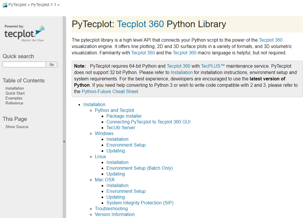
Documentation and installation instructions are available on our PyTecplot page.

PyTecplot is a Python API available to use with Tecplot 360 (with a maintenance agreement). More information, such as documentation and installation instructions on PyPi.org are available on our PyTecplot page.

PyTecplot runs in two modes:

1. Connected-mode drives a live-running Tecplot 360 instance
2. Batch mode is helpful if you have many files you want to process on a cluster. You will need enough licenses to run multiple instances simultaneously. But this powerful tool gives you access to the raw data.

Python is a separate installation. Please read the installation instructions. If you have Python 2.7, 3.4 or 3.5 and newer you can use PyTecplot. The command is “PIP install PyTecplot” on most machines.

First, I will reset the plot with CTRL+F and turn off the mesh.

Probe On Surface Demo

Video Timestamp – 0:19:30

I am going to run a script that I have already written, and then I will show you how it works. 

1. To allow a Python script to drive a Tecplot 360 instance, we need to connect PyTecplot. Select Scripting>PyTecplot connections and make sure the Accept connections box is checked. We use sockets to communicate in between Python and Tecplot 360. In this demo, we are communicating with sockets over port 7600.
2. Second, bring up a command prompt, and run the script, ProbeOnSurface.py.
3. This script will find the XYZ locations for each of the zones that defines the points. At each location, it will call the Python script probe_on_surface and then construct a new zone within Tecplot 360.
4. To confirm this, open the Data>Data Set Information dialog. You can see that we have the probed values.
5. Open the Zone Style dialog and turn these zones on.
6. Change the scatters symbols to cubes and change the size to 1.5%.

Now you can see the measured values are close to the spheres. Zooming in again, we see that the cube is actually on the surface, whereas the measured location is slightly off the surface. But using the normal of the cell to identify the closest location to the sphere is as close as we can get. Zoom back out using CTRL+F.

Analyzing the Probe On Surface Data

Video Timestamp – 0:21:30

Now we want to analyze this data. Let’s look at the data in a line plot.

1. Create a new frame.
2. Set the Plot to XY Line. The new plot inherits the data from the original plot.
3. In the Create Mappings dialog, set X-Axis versus Y-Axis for all linear zones. And we want to look at X vs Pressure_Coefficient.
4. Open Plot>Axis and reverse the Y-axis for the proper orientation of the Cp plot.
5. Now let’s focus on one of the sections. Open the Mapping Style dialog and select only Map Number 4 and 11 (Sections 4 – .8),  and check Show Selections Only.
6. Then fit the plot with CTRL+F.
7. Add the line legend with Plot>Line Legend and click the Show Line Legend checkbox. Check the Symbols checkbox.

Now I have a quantitative view of the data. You can see the area where there is a large variance between the simulated data (probed line) and the measured data.

Analyzing the Variance Between Probed and Measured Data

Video Timestamp – 0:22:41

How do I find the variance on the model? Let’s bring our 3D view to the front and then do a calculation to highlight where the variance is.

• In the Zone Style dialog, let’s again just focus on 0.8 and show selected only, and turn our wing back on.
• Select Data>Alter>Specify Equations
• You can see my seeded equation {cp_diff} = V12[6] – V12. This will compute a new variable called cp_diff. This will be the difference in pressure coefficient between the 12th variable in my dataset. V12 is shorthand for the Pressure_Coefficient. Make sure that you select zone #13 in the zone list because we want this equation to apply only to that zone.
• Press Compute to calculate the difference in coefficient of pressure between these two zones.
• Color the cubes by that difference in pressure coefficient. Open the Contour dialog and set up another contour group for cp_diff. Set the levels from -0.1 to 0.1 with 11 levels. This will put zero right at the center.
• Select a different color map. I will choose this orange and purple.
• Open the Zone Style dialog, right-click and select contour group 2. Now you can easily see where we have a difference between our measured data and our simulated data.

The scatter symbols are sized by a percentage of the frame. In Tecplot 360, you can zoom in on the frame itself. You can see I am bringing the whole frame closer to me. To do this, I am holding down the shift key and pressing and dragging the middle mouse button, that brings everything closer. Now I can get a quantitative understanding of the difference between the measure data and the simulated data.

The Python Script, Probe On Surface

Video Timestamp – 0:25:55

To fit all my frames back to my view, press CTRL+Shift+A, and to fit my wing, press CTRL+F.

Now, let’s look at my Python script, ProbeOnSurface.py. The script is available in the packaged download file.

• Import a Python package called NumPy, which is a mathematical package. NumPy has functions for matrices, arrays, and other mathematics.
  import numpy as np
• Import the Tecplot package and alias Tecplot to tp. Everytime you see tp, I am referencing Tecplot.
  import tecplot as tp
• Connect the script to the live running version of Tecplot 360.
  tp.session.connect()
• Suspend the user interface. Because I am connected to a live running instance of Tecplot 360, every function call will try to update Tecplot 360. In this situation, because I am doing introspection of the data and math, I don’t need to update the view until the end. Suspending the user interface will make the script run a little bit faster as well.
  tp.session.suspend():
• Get the current frame.
  frame = tp.active.frame()
• Get the dataset in that frame.
  dataset = frame.dataset
• Get a list of zones that start with the word “Section.” This is my measured data. (My measured data all start with the word “Section.”)
  sections = dataset.zones(“Section*”)
• Loop over all Section zones, which puts the XYZ locations associated with my measured data into an array.
  for zone in sections:
      print(“Extracting simulated results for: “, zone.name)
      points = [zone.values('x').as_numpy _array()
             ,zone.values('y').as_numpy _array()
             ,zone.values('z').as_numpy _array()]
      num_points = len(points[0])
• Pass this data off to the Probe On Surface function. Limit the search to a single surface to make sure that Probe On Surface looks only for data on the wing surface.
  res = tp.data.query.probe_on_surface(points, zones=[dataset.zone("WingSurface")])
• Through a little bit of NumPy magic, I can reshape the results, so they are passed back off the Tecplot to create new data.
  values = np.array(res.data).reshape((-1, num_points))
• Add a new zone to the dataset with the probed results (called “Probed -“). Do this for each variable. And then for each of the variables in the dataset, I am putting the probe results into this resulting zone.
  probed_points = dataset.add_ordered_zone('Probed - ' + zone.name, num_points)
  for val, var in zip(values, dataset.variables()):
        values(var)[:] = val
• End the script.
  print("Done")

If you are new to Python and PyTecplot, our PyTecplot Docs are a good resource, and if you have a Tecplot license with maintenance, contact our excellent Technical Support Team.

We will be posting the Q&A section of this Webinar in a separate blog.

Get the Newest Version of Tecplot 360

Request a Free Trial

Get Invited to Upcoming Webinars

Subscribe to Tecplot

Related Videos