Thermal Field Visualization for Uncertainty Quantification of the Material Melt Pool in a Selective Laser Sintering Manufacturing Process
Contributed by Nicolas Castrillon, Ph.D. Candidate, Mechanical Engineering, University of California, Berkeley, UC Berkeley MSOL website
Additive manufacturing (AM) has been permeating the industrial fabrication space for decades. Technologies that encompass AM are vast: some examples include fused deposition modeling, selective laser sintering (SLS), and material jetting. Due to the nature of these processes, controlling the print quality everywhere in the final printed part is a hard problem since different regions of the part are printed minutes to hours before other regions and so external (for example, environmental) effects can change during that span of time.
Quantifying the Amount of Uncertainty
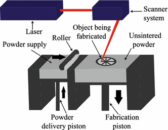
The SLS process is greatly affected by uncertainty sources that are in nature and which ultimately contribute tremendously to the quality of the printed part. In this study the aim is to quantify the amount of uncertainty that arises from printing a SS 316L part via the SLS process. The SLS process consists of using a thin laser that scans the top of a bed of powdered material in order to melt and consolidate local powdered material and ultimately print a part layer-by-layer. Figure 1 shows a schematic of the SLS printer. Uncertainty of the extent of material that melts and consolidates arises from the random arrangement of particles with a radius that obeys a particle size distribution function. It is the local arrangement and size of the particles the affects the amount of laser energy that is locally absorbed by the material and that permeates the powder layer into the underlying, previously-solidified material substrate.

Figure 1. A schematic of the selective laser sintering (SLS) process [1].
Simulating the Laser Scan Path
A single track of the laser scan path is simulated, and the thermal equation is solved via a coupled finite difference – discrete element method. The solution of this simulation is to be used later in a downstream step for capturing and analyzing the size of the material melt pool both in space and in time, thus measuring the variation of the shape of the melt pool. Figure 2 shows a video of the simulation using Tecplot 360 where a laser scans the top of the domain in the +x direction. On the top-right corner we see that an x-z cross section has been taken to provide a better visualization of the thermal field into the substrate. A top view is also provided on the bottom portion of the video.
Figure 2: Video of Tecplot 360 simulation where a laser scans the top of the domain in the +x direction.
Leveraging Tecplot 360
Tecplot 360 has been crucial in the debugging phases of my Python implementation. Each time I run the simulation I write the temperature field values in IJK point files, which I can quickly load up for visualization by using a previously saved layout file and a frame style file. In this way, loading new results with small data files is effortless (less than 1 GB).
Posterior to the debugging phase, running the simulation with a finer grid generated ASCII .dat files that were about 80 GB in size. Using the Preplot functionality as a post-processing step I can convert the ASCII .dat files into binary .plt files, reducing the file size to about 15 GB! Tecplot 360 loads these binary files almost immediately.
I was a ParaView user for several years and I always struggled with loading large file sizes and manipulating the visualization. Tecplot 360 blew me away as it allowed me to say good-bye to the days of crashing data visualization software.
– Nicolas Castrillon, Ph.D. Candidate, Mechanical Engineering, University of California, Berkeley
Learn more about Tecplot 360 »


