Tecplot for CONVERGE Tips, Tricks and Tutorials

Tecplot, Inc. and Convergent Science formed a partnership in June 2018 to distribute (to all users of CONVERGE software) a version of Tecplot 360 called Tecplot for CONVERGE. This blog starts with an introduction by Tiffany Cook, Partner and Public Relations Manager at Convergent Science. Then Scott Fowler, Tecplot 360 Product Manager, will talk briefly about Tecplot products and services. The rest is a tutorial for using Tecplot for CONVERGE.

Convergent Science

Speaker: Tiffany Cook

All right, Scott, thank you. For those who are not familiar with Convergent Science, we were established by graduate students at the University of Wisconsin in Madison. Three of the owners are at our home base, or headquarters, which is also located in Madison, Wisconsin.

We have offices in Texas, Michigan, Austria and India, in addition to distribution in Asia through our collaboration with IDAJ. I’d also like to add, trainings in the US and Europe are free of charge, and we do offer licenses to universities at a reduced or zero cost.

As Scott mentioned, we joined forces with Tecplot in June of this year, and we’re just really excited about the partnership. With our partnership, CONVERGE users have access to Tecplot for CONVERGE at no charge, so as you learn more today, we definitely encourage you to take advantage of their post processing capability.

To further give you a little bit of background about CONVERGE CFD, we pride ourselves on its key feature, which is AMR, adaptive mesh refinement, and that basically eliminates the grid generation bottleneck from the CFD simulation process. And if you’re familiar with our code, you know we’ve done quite well in the internal combustion engine area, but CONVERGE can also be applied to the application areas that you see here. And along with the benefits indicated, CONVERGE also has various options for chemistry, spray models, combustion models, emission and turbulence.

CONVERGE has been commercially available for about 10 years, and at this point, approximately 95% of U.S. engine manufacturers use CONVERGE, and 85% of engine makers in Europe and Japan are using CONVERGE. So you can see that our reach is beyond the U.S. We are a global company.

We are in the process of completing CONVERGE 3.0, which will have significant improvements in scalability and boundary layer meshing. The estimated release date is early 2019.

Finally, I’d like to mention that we also have an upcoming webinar next Wednesday. It’s focused on after treatment, so I’d like to invite you to visit our website, check out our resources and also upcoming events to get more detailed information on CONVERGE. www.convergecfd.com.

And with that being said, I will turn the control back over to Scott.

Speaker: Scott Fowler

Great. Thanks Tiffany. I would like to also mention that we are very happy with the partnership with Convergent Science. It’s been a great, and we’ve certainly learned a lot about internal combustion engines on our side, and we are excited to move forward and to provide great software to users of CONVERGE.

Tecplot, Inc. at a Glance

Tecplot was founded in 1981 by a couple of Boeing engineers. Our background is largely external aerodynamics. We are the largest independent CFD post processor in the world, with approximately 47,000 users worldwide.

We’re known for being the most complete and flexible post processor, which I hope you’ll see today through our ability to do not only high quality 3D plots like you can see here on this slide, but also 2D and line plotting, with a lot of control over what you can do with the plot.

We are also trying to be very responsive to CFD community. We see dataset sizes are growing, people need to do more comparative analysis, so we’re working on techniques and tools for handling those needs.

We are trusted worldwide by some of the largest companies, particularly, you can see a lot of influence in aerospace, but we also do have some seats in automotive with Honda and Fiat, GE being used for the gas turbine section.

Tecplot 360

And just a quick tour of our products. Tecplot 360 is our flagship product. This is what Tecplot for CONVERGE is based on, and this is what you’re going to see in the demo today. So this is our primary tool for looking at CFD and test data.

Chorus

Chorus is available if you purchase a fully licensed version of Tecplot 360. Chorus helps you explore large datasets for multiple simulations, and compare those results. So if you’re doing an ensemble analysis, this is going to be a nice tool for you.

PyTecplot

PyTecplot is a Python API that we released in early 2017. PyTecplot is available with the full version of Tecplot 360. It’s also available with Tecplot for CONVERGE. The one limitation is, in Tecplot for CONVERGE, you cannot use this in batch mode. PyTecplot really offers a lot of additional capability, and has allowed many of our users to do advanced analysis that they weren’t able to do before. It gives you full access to the raw data behind your simulation, so you can perform interesting calculations and automate workflows. You can see here that, compared to the Tecplot macro language when doing a complex mathematical operation, we were able to get the speed from 18 minutes down to 7.3 seconds. So quite an advantage there in using the Python API.

Tecplot for CONVERGE

What is Tecplot for CONVERGE? Tecplot for CONVERGE is effectively Tecplot 360 with just a few minor limitations. It is included with your CONVERGE Studio license, so if you do need access to Tecplot for CONVERGE, Convergent Science can give you access to the download and license for Tecplot for CONVERGE. Like Tiffany said, it’s free of charge with your purchase of CONVERGE and access to CONVERGE Studio.

Tecplot for CONVERGE is a nearly full featured version of Tecplot 360. The limitations are:

• No batch mode operations. If you do need to use batch mode, you will have to purchase the full version of Tecplot 360.
• Limited to one page and five frames. If you’re not familiar with those terms, you will see them during the demo.
• Loads only data produced by CONVERGE.

So, we want CONVERGE users to have a very full-featured, a very performant application, and that’s what you’re getting with Tecplot for CONVERGE.

Here are the differences in a table. Tecplot for CONVERGE has a small watermark, license and download is all from Convergent Science. The scripting is available in the GUI (graphical user interface) only. If you do upgrade to the full Tecplot 360, you will have access to batch mode. And then one of the key things here is, the bottom line, number of CPUs that Tecplot for CONVERGE uses, we put no limitation on that. So you can use all the horsepower you have available on your workstation.

Tecplot for CONVERGE Tutorials

Now I’ll jump into a demonstration of Tecplot 360. And again, everything that I’m going to show you today can also be done in Tecplot for CONVERGE. So we’ll go through working with CONVERGE data. I’m going to be using an internal combustion case, like the one that you see in the plot here.

One of the critical things is that you do have to use post_convert to convert your data to Tecplot format. Use the most recent version of post_convert you can get, because we do put a little checksum in the files to ensure that the files loaded can be loaded in Tecplot for CONVERGE. So if you have previous Tecplot PLT files that you had created, those may not load in Tecplot for CONVERGE, so just make sure that you’re using the latest post_convert.

In this demo, you will how to:

• Use slices and iso-surfaces
• Display parcels
• Compute mass flow rate
• Use cell average output files
• Export images and movies

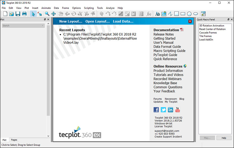
Tecplot 360 User Interface

If you haven’t seen the user interface before, I’ll just give you a quick tour. When you launch Tecplot 360, you see in the middle here what we call the welcome screen. There are some really nice resources here, particularly the documentation and the Quick Reference Guide. There are a number of keyboard shortcuts and mouse shortcuts that are going to be useful for streamlining your work flow. So please take a look at the Quick Reference Guide in our Documentation.

Online Resources

• Getting Started with Tecplot for CONVERGE Webinar
• Tecplot for CONVERGE Video Tutorials
• Tecplot 360 Documentation
• Tecplot Technical Support
• Convergent Science Technical Support

If you do have any questions or need help, you can always contact support@tecplot.com. The support staff at Convergent Science are also trained in Tecplot 360, so you can start there as well. So, please, do come back to this welcome screen. If this welcome screen is not visible, you can always get to it by going View > Welcome Screen.

Loading Data

Let’s start with loading some data. I’ve already run this data through post_convert, so I’ll just go File > Load Data. I have here 145 time steps, ranging from crank angle -381 all the way to crank angle 340. This is total about 12 GB of data, and just to give you a frame of reference, the machine that I’m on is an 8 core, or 8 CPU laptop with about 32 GB of RAM. It’s about three or four years old. So it’s not exactly state of the art, but I think that you’ll see that the performance is quite good.

Now that we’re in Tecplot and we have the data loaded, just a couple of terms. We have, in the middle area, we call this the workspace. We have what we call here a frame, and a frame contains the data and will result in a plot. On the sidebar here, we have what we call the plot sidebar. So this will affect the look and feel of your data. And you’ll see me use these throughout the presentation today.

Data Set Information

One of the first dialogs that is critical is the Data Set Info dialog. And this will let you know what data we have loaded. You can see that I have what’s called a zone. A zone is simply a collection of data. So zone number one is my CONVERGE volume cells, the grid that’s produced through that adaptive mesh refinement technique that Tiffany was talking about. You can see that this zone is of type polyhedron, these are volume cells, with about 127,000 elements, at solution time, or crank angle, -381.

These zones are also given another identifier called a strand, and this is going to be important later in the demo. Strand ID of one, a strand is just a way of describing a like set of data through time. So you can see the grid, the volume cells, are assigned to strand one. If I go down to another crank angle, it’s still assigned to strand one at a different crank angle.

Same sort of thing for boundaries. Boundary number one is assigned to strand number two. If I go down, boundary number one again, strand number two. So this is just a way to identify like data through time.

Another interesting thing that you’ll see here in Data Set Info dialog is the variable information. This says variable status not loaded. Tecplot has actually not gone through the effort of loading this data yet. We use a technique called Load on Demand to reduce the amount of RAM required to generate a plot. In this case, the only information that we need to display are the surfaces, or the boundaries, so none of the information for the volume has actually been loaded yet.

The rest of the data will get loaded when we add a slice or an iso-surface. Keep in mind that, while it says not loaded, it is available, and Tecplot 360 will load it as it’s needed. Tecplot will also unload data as it’s no longer needed, to reduce the memory footprint on your machine.

Zone Styles

Let’s also bring up what we call the Zone Style dialog. This is also a critical dialog for setting the style of your plot. And you’ll see that there is quite a lot of similarity in what we have in the Data Set info and the Zone Style dialogs. There is a much shorter list of zones. So again, the grid is all strand number one, and so this is just in this first entry. So as I advance through time, you can see the Zone Style dialog advances. And so we can see that what we’re actually seeing in this plot is, or are the zones associated with crank angle -365.

So that’s a quick demonstration of the Zone Style dialog and Data Set Info dialog. Again, the asterisk here indicates that these are zones through time. We will come back to those dialogs later in the demo.

Slices (and Keyboard Shortcuts)

Let’s take a look at this dataset. One of the first things that we want to do, is inspect the mesh that CONVERGE creates, and a great way to look at that adaptive mesh is through slices. So let’s go ahead and put in a slice. I’m going to use the Slicing tool.

I can just click on the plot, and click right in the middle. I’ll just tell you a couple of keyboard shortcuts here. For rotation, you can use the rotation tools in the ribbon, or just hold down the CTRL key and right click, and I can rotate the plot around.

Now I can’t see the slice very well, so let’s turn on translucency. I actually want to see the interior, so we will use a setting called Value Blanking to see the interior. Select Plot > Blanking > Value Blanking, and we’ll say when X is greater than zero, and we’ll turn that on. And now we can see the interior of this cylinder.

Zooming in and out is done by holding down the middle mouse button. Translation, hold down the right mouse button. Rotate, CTRL and right mouse button.

Now, if I want to set the center of rotation, rotating this around, I can just hover over, and I’ll hit the O key on the keyboard. This is a really critical thing, so now I’m rotating about this point. If I want to rotate about this point way on the left, I hit the O key over here, and you can see it’s rotating around that. So the O key is a really critical keyboard shortcut.

Again, go back to the Welcome Screen and look at that Quick Reference Guide, and you’ll see all those shortcuts.

Adaptive Mesh

Now let’s say I want to look at the mesh. I can simply right click on that slice, and toggle on the mesh. Let’s say I want to look at temperature on this slice. I can just use this toolbar and select Temperature. And now let’s go ahead and we’ll just advance through time, and we can see how this adaptive mesh develops as we’re going through our simulation.

Iso-surface Details

Another thing that we may want to do is look at an iso-surface of a particular temperature to visualize the flame front. So let’s go ahead and pause this animation.

Point of note here, it says drawing interrupted. There are two ways to get out of this. One, you can just click Redraw on the sidebar here, or middle mouse click will also perform a redraw, as just a quick shortcut. Anytime you hit Pause, or sometimes if a redraw is taking a long time, and you want to continue doing your work, you don’t have to wait for the redraw. You can just keep clicking, but it will interrupt that redraw.

We want to look at an iso-surface of the flame front. So, let’s define that using the Iso-surface Details dialog. We want to do an iso-surface of temperature, and let’s say we want to do a specific value of 1500, and we’ll toggle this on to display it.

And you can see, we have another contour legend on the plot. This iso-surface is being contoured by mass, but let’s say we want the contours to be by temperature as well. And we see no iso-surface at this point. The iso-surface at this point is not quite at the combustion phase, let’s just move in. And we can see the start of the iso-surface here. As we advance through time, you can see this iso-surface is getting clipped by the value blanking, but we want to see the entire iso-surface. On the Iso-surface Details dialog, we have this option says, “obey sources of blanking.” The volume-cell zone that this iso-surface is going through is being clipped by the value blanking constraint. We want to turn this off so we can see the full iso-surface. Now it’s not constrained by that value blanking. And again, we can animate through time and see that flame front develop.

Plot Annotations

Okay, now let’s do a couple of other things here. Let’s say that we want to see the entire boundary again, so go in and we’ll turn off the value blanking constraints. And I want to know what crank angle we’re at while we’re on the plot. I can use plot annotations. Here I’m using a text annotation tool (Text Details Dialog) and I’m going to type Crank: &(SOLUTIONTIME) And then I’ll use a piece of what we call dynamic text. This is text that’s going to update as we’re animating through time. And we’re going to say solution time. And then we hit Accept, and then as we add advanced through time, this piece of text is going to update.

Now we do have some flexibility here in the formatting. I don’t need that many digits of precision, so I’ll add to the plot annotation Crank: &(SOLUTIONTIME%0.2f) and we’re now limiting it to two-digit precision. Nice way to get an annotation on the plot.

Parcels

We’ve briefly talked about slices, we’ve briefly talked about iso-surfaces, little bit of rotation and keyboard shortcuts, translucency. Let’s move on to showing parcels. This simulation does have spray in it. We’ll go ahead and turn off our iso-surfaces and our slices. And now this is where we’re going to come into the Zone Style dialog and deal with the zone layers.

We’ll launch Zone Style dialog. And we see that, we do have a zone here called spray and in order to visualize this, we need to show scatter. The scattered layer. Scattered plot and layer is what we want to look at here, you can see the Tecplot has turned the default to show scatter for everything, we want to show it only for the spray zone. Go ahead and select all of those, turn it off for everything but spray. And then we can toggle it on here on the sidebar.

Now we can see our particles. The default is square. I prefer points in this case, so let’s change it to points. And let’s say we want to color these by a specific variable. We can do that as well. We’ll go in to the outline color – just a note, I’m right clicking on these columns to make the selection – so it’s a right click. This launches a dialog and I’m given a color chooser and I want to use multiple and multi-color option or a contour color. Now I’m going to have to select multi 1, 2, 3, 4, 5, 6, 7, 8. What does that mean? This is associated with what we call the contour details. Anytime you’re using multi-color, it’s important you understand contour detail. Let’s go ahead and close the Zone Style dialog and launch the Contour Details dialog.

I currently have my contour groups here, let’s assign contour group 1 to DP_film_flag. That’s what I’m going to color these particles by. And I know that film flag has values from zero to five, I’ll go ahead and set up my contour levels this way: min, max and a delta. And through playing with this I know that qualitative dark two is a nice color wrap to use when coloring by film flag. Okay, now I’ve set up what we call a contour group, with a specific type of coloring you can see earlier when I was using temperature that’s associated with contour group 3. Now I can right click here, select multi 1. And these are now colored by film flag and I have a contour legend that has been displayed showing my values.

Let’s back up to right around when those particles had the sprays injected, and as we advance through time here, we can see the propagation of the spray and we can see how the film flag value changes.

Let’s say I want to isolate particles that have a specific film flag value. Again, this is where we can use value blanking. We’ll go back into the Value Blanking dialog and select DP_film_flag not equal to zero. This will show me only the particles (or spray) that is “not in the wall film”. If we want to look at the particles or spray that are only in the wall film, we can assign a value of one.

Macros

You may not always remember the meaning of each one of these values 0, 1, 2, 3, 4, 5. This is where you can use Tecplot scripting capabilities. We have what we call the Quick Macro Panel and you can see that I’ve added a few things that are specific to CONVERGE data.

Our macro language is pretty robust. We have a way to prompt for instructions, that’s what we’re going to do here. I’m going to double click on Show specific parcels, and this pops up a little prompt dialog that says, “enter the parcel type to display.” And I’ve entered some strings here to help me remember what each one of these values means. If I want to look just at my rebounded particles, I can just hit the value two and when I hit okay notice that the Value Blanking dialog updates as well.

Now I’m looking at only the rebounded parcels or if I want to go back to looking at the ones that are not in the wall film, hit zero. If you have repetitive tasks or have just a couple of buttons that you don’t remember how to use very often, you can use the scripting language and register some commands right over here on the Quick Macro Panel, that’s a nice feature to use.

Instead of just using points for parcels, we may want to use spheres. Spheres are more expensive to draw; you’ll see the redraw speed does slow down a bit here. We’ll say spheres and then I want to size these, say by their radius. Select a variable, select DP_radius and then finally assign it to DP_radius.

You can see that the particles are quite small and let’s turn off the value blanking so we can see more of the more of the parcels. You can see we have some larger radius spray particles up here at the injector, and as we advance through time it’s going to advance a bit slower now because those spheres are a bit more expensive to draw, but they do make a great looking image for final presentations.

You will see that this animation did speed up a little bit. That’s in part because data have already been loaded for these time steps, we do cache data in RAM as much as we can. And we also have a smaller grid up here at top dead center and fewer parcels, it’s just less work for the graphics card at that point.

Computing Mass Flow Rate

Let’s move on to doing some more analysis. We’ll look at how to compute mass flow rate. This is going to involve slices again. Let’s go ahead and turn off scatter, value blanking is turned off. And what I want to do is, I want to look at mass flow rate and what we’re going to do, is we’re actually going to compare it to results that were produced by CONVERGE itself. If I click here you can see that I have boundary even selected, I do have a CONVERGE output file that has mass flow rate for this boundary. We’re going to compute mass flow rate in this region.

To do that, we have to place a slice. Tecplot will operate on, will do analysis on, the zones only. The slices are what we call derived objects, we can’t actually perform calculations on those slices, we have to extract them to zones.

Let’s first place this slice. I have a slice here, and I want it to be aligned with the boundary. I’ll choose the Slice location as Arbitrary. And then I can use a 3-Points probe tool to get it to align with that boundary. And then I’m going to move it in, just a little bit to make sure that I’m cutting through the volume cells.

Again, we need to compute the mass flow rate, but we need zones. If I go back into Data Set Info dialog, you can see I don’t have, slices don’t show up any anywhere here. These are a transaction object. We need to make these an object that is static, for lack of a better term.

We’ll go into Data > Extract > Extract Slices Over Time. This is going to step through each time step. It’s going to slice that volume mesh or the volume grid and it’s going to extract or create a zone out of these slices. It should take about a minute, to a minute and a half to perform.

I’ll bring up the task manager in windows here. You can see that we’re using a large amount of CPU here. You have access to all the cores on your machine using Tecplot for CONVERGE and you can see the memory is climbing as we’re loading the data required to do this extraction. And again, Tecplot will manage this memory for you. Those previous time steps, -381 up to top dead center in that region that are not currently needed for this plot. If we were to run out of memory or get close to the memory limit on your machine Tecplot will start unloading that memory. We do a pretty good job of managing the RAM for you.

This is just a few steps from done and then we’ll be able to move on to the actual mass flow rate calculation. Alright, we’re done. Now if we go into Data Set Info dialog and scroll all the way to the bottom, you can see that we have new zones FE – Polyhedron. These are surface cells and we have one for each time step. And you can see that they have a new strand number. So each one of these is going to be associated with the same Time Strand. So again, a grouping of data through time is a Time Strand.

You can also see this show up in the Zone Style dialog. We’ve extracted those, it’s not enabled by default, but if we turn it on, you can see that it’s coincident with the slice. We’ll just go ahead and turn that back off. To compute mass flow rate, we go into the Analyze menu and we’re going to say Perform integration and select Mass Flow Rate. We’re going to choose, Integrate by: Time Strands. This is going to integrate across all of those slices through time. We’re going to select those slice zones that we just created. And we’re going to set Plot Results As to Mass Flow Rate. I’m going to hit Integrate, and it’s going to give me an error and I’ll explain the error.

Error: The current field variables don’t define the required convection variables. Please set them in the Field Variables dialog.

In order to compute mass flow rate, we need to know convective and state variables and that’s available here under Analyze > Field Variables. We need to do the following:

• Define our velocity components u, v, w
• Select pressure and temperature
• Set the proper gas constant: Analyze > Fluid Properties
  For this dataset we’re using 287.

Now we’ve given all of the information we need to compute mass flow rate, and we can simply hit Integrate. It goes through this process quite quickly, and we get a new plot that shows us our mass flow rate at this location.

As I move over to this line plot, you can see our plot sidebar changed. It says that we’re in XY Line mode, and we have a number of attributes showing line symbols. Again, we can right click on the plot and toggle the symbols off and make the line little bit thicker. Let’s go up to point four so we can see that a little better.

As we advance through time, you can see a timing mark that moves to show where we are in relation.

I want to compare this to the results that CONVERGE creates. We will open up another file we’re going to append data to this frame. Earlier in the presentation we talked about pages and frames you’re limited to one page which is one work area here and five frames in Tecplot for CONVERGE. In this plot I have two frames. You can see you can get quite a lot of work done within those limits, one page and five frames.

Let’s load the CONVERGE output file, area_avg_flow.out. Tecplot 360 has a number of different loaders. You will probably not see this dialog with Tecplot for CONVERGE because it has fewer loaders.

Tecplot 360 asks us if we want to replace the data or if we want to append the data, and we want to append the data to this frame.

The CONVERGE file has a different variable names than what we had currently loaded in the dataset. We need to tell Tecplot which variables mean the same thing, in this case we need to Combine:

• Crank (DEG) = 1: Solution Time
• Mass Flow Rate (kg/s) = 2: Mass Flow Rate

The rest of the variables don’t need to be imported at this time. I’ll just go ahead and hit OK.

You can see that the plot labels changed and let’s see what is available in Data > Data Set Info. You can see we a couple of new zones and we will clean up the zone names (double click to edit). Strand 169 – these are the results of the Mass Flow Rate. Then we have variables, and let’s clean up the variable names to Crank (DEG) and Mass Flow Rate (kg/s). Average area flow bound ID 7 (area_avg_flow_bound id_7) is what I want to plot in the line plot to compare the computer to CONVERGE result.

To do that, will go into the Mapping Style dialog. This is a lot like the Zone Style dialog but for line data. We have one line-map available right now, we’re going to create a new line map to show Crank vs. Mass Flow Rate for zone 2:area_avg_flow_bound id_7, which is the boundary ID at this location, I’m going to use a key word here called “&ZN” to call the map by the zone name. You can see the map name captures zone name.

In the line plot, turn off the symbol layer. I’m going to do CNTL F to fit the data. And you can see that we have pretty good agreement with the output from CONVERGE if we zoom in close and we turn on the symbol layer again, you can see that we have a lot more resolution in the data.

We have a lot of control over the symbol shapes. Let’s change both of these to circles, make them quite a bit smaller and fill them. Then, we’ll fit again using CNTL F. You can see that we have a lot of control over the plot and over the axis, as well. You have interactive control with the label – you can see the label is overlapping the title – so we will use our adjuster tool and move the labels.

Let’s say I want to get his plot ready for final presentation. We can disable the background, hide the border, and resize the plot. Let’s move the legend out, and then we’ll zoom out. Now we have a multi-frame plot, and we can then animate this to a file.

Let’s go into Solution Time > Details. You see we have this film strip icon, we can select a number of different movie formats (AVI, Flash, MPEG4, Raster Metafile, WMV):

• MPEG4 seems to be the most portable. I would encourage you to use MP4
• Specify width – 1024 is a nice width.
• Use what we call, anti-aliasing which will smooth out any lines.
• Specify animation speed.

I’m not going to hit okay right now because it takes about eight minutes to render this to a movie file. But you can see that you do have the various export formats for creating movies.

If you wanted to create just a still image of this, go to File > Export, and there are a number of raster and vector export options. The most common is PNG for the raster formats. For the vector formats, PostScript or EPS work quite well. WMF works very well on Windows platforms. Quite a lot of capability there.

I did generate a movie earlier. So, let’s just bring that up and we can show you an animation created with this data. Again, this took about eight minutes to render on this machine.

Macro and Python Scripts

Let me finish up the presentation with a brief discussion of macros, Python scripts, and other various file formats that we have. We did a lot of work to create this plot. Let’s say we don’t want to redo all the point and click effort every single time. You do have the ability to record Python and macros under the scripting menu. The Tecplot Macro Language is a pretty easy to understand human readable language. We’ve done a great job with Python over the last few years. You do have a couple of different options for scripting.

Again, Tecplot for CONVERGE allow these scripts to run from the user interface with the GUI up. If you do need batch mode scripting, then you will have to purchase a full version of Tecplot 360. Please keep in mind that you do have the ability to do scripting, just not in batch mode.

If you want to save your work, there are a couple of different ways to do that. You save a layout, which will save the state of everything you have here. But layouts if you do a slice extraction like we did here will “dirty the data”. So, it will ask you to write out the dataset. In that case, a better option may be a combination of macros and style sheets. Again, a layout is going to save the state of all the frames. Here we have two frames, and it’s going to retain links to the data. A style sheet is going to save the state of just one individual frame. So there are a couple of different ways to save your work.

I really like our Python layer. Let me show you one of the really neat things you can do with Python. I’ve registered a Python script on the Quick Macro Panel. This Python script actually constructs a small user interface using PyQT. It interfaces directly with Tecplot 360:

• Add Crank Angle. We added crank angle on the plot earlier. Let’s say I don’t want to remember the keywords for adding crank angle to the plot. Well, I built this little user interface I can just click Add Crank Angle and it adds the crank angle.
• Add RPM of this simulation; I can get it in one click.
• Jump to Crank Angle. Let’s say I change Solution Time pretty frequently, and I always know I want to go to a bottom dead center. Just type -180 and jump to that crank angle.
• Parcels to Show. Let’s turn scatter back on here. Here I have a nice drop down that says, let’s show just the ones that are in the wall film. So, again, this behind the scenes is changing those value, blank, and constraints. Let’s say I want to go back to see all of them.

You can do quite a lot with the Python layer that you can’t do with macros. Macros are great for simple scripting. Python is great for, not only complex user interfaces like this but, if you want to integrate with other tools or do advanced analysis, deal with the file system, Python API is really great.

Conclusion

There’s a lot more that you can do with Tecplot 360 and I encourage you to ask questions of Tecplot, Inc. and Convergent Science, on how to use Tecplot for CONVERGE.

Just to round out, we are focused on solving the big problems in CFD post processing. Tecplot 360 can process large datasets very quickly using all the CPUs on your machine and our load on demand technology.

Tecplot Chorus, which we did not demonstrate today, but we do have a number of webinars and videos on our website for Tecplot Chorus. That’s for ensembles or multiple simulations.

You saw a pretty good demo of PyTecplot and what you can do with it. Again, Chorus and PyTecplot are included with the full paid version of Tecplot 360. If you are interested in upgrading to the full version of Tecplot 360, we do offer discounts for CONVERGE users. I encourage you to contact our sales team to inquire about that.

Request a quote for Tecplot for CONVERGE

With that, I’d like to again, thank Tiffany and Convergent Science for being a great partner and allowing us to provide great post processing tools for the CONVERGE community.

Check out the Q&A from this webinar.