


 MENU
MENUVisualizing Higher-Order Finite-Element Data – Part 2: The Challenges
This blog was written by Dr. Scott Imlay, Chief Technical Officer, Tecplot, Inc.
“Run when you can, walk if you have to, crawl if you must; just never give up!”
-Dean Karnazes, Ultramarathon Man
I feel it is important to acknowledge our worldwide struggle with COVID-19. Like me, most of you have probably made significant changes to your lives to slow the spread of the disease. Some of you have been more directly affected; having yourself or loved ones fall ill. A few of you may have lost a loved one. I used variations of the Dean Karnazes quote above as a mantra to help keep me moving through the most difficult parts of IRONMAN triathlons. It also helped me through the darkest moments of my grief after my daughter passed away last year. If you are going thru a dark time, give it a try.
Run when you can, walk if you have to, crawl if you must, just never give up! Keep moving forward!
Visualization techniques for Higher-Order Finite-Element Solutions
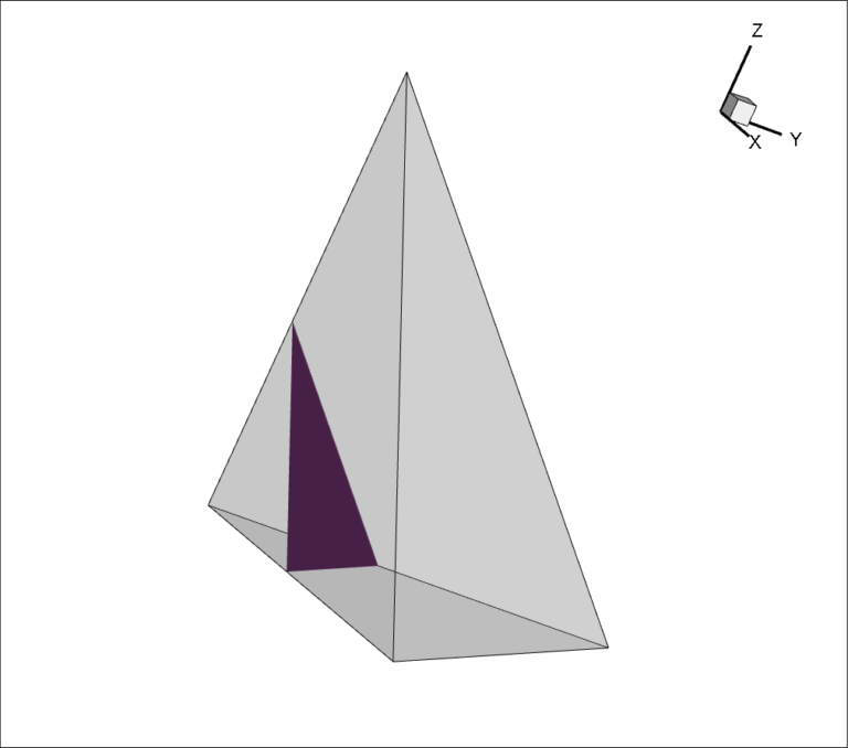
Figure 1. Isosurface in a linear tetrahedra.
In keeping with this theme, my colleagues and I at Tecplot are pushing ahead at full speed on new features and new releases, in spite of working from home. My current role is researching visualization techniques for higher-order finite-element solutions. My last blog Visualization of Higher-Order Elements was a primer on higher-order finite-element CFD methods – what they are, how they are used, and what they work best for. In this blog I will address the challenges visualizing the results of a high-order CFD solution.
The complexity of higher-order finite-element data complicates the visualization process. First, is the variability in defining the coefficients of the polynomial basis functions. For nodal techniques, the coefficients of the basis function are the values of the solution at the nodes. Sometimes a modal technique is used where the polynomial is less coupled to the nodal values. When developing visualization algorithms for the higher-order-element data we much decide which basis functions to use.
Frequently, the polynomial order used for the solution is higher than the polynomial order used to define the curved edges and surfaces of the grid. For example, the grid may use a linear or tri-linear polynomial (our normal elements) while the solution within the element may vary by a third-order polynomial. For curved edges and surfaces, a second- or third-order polynomial is often used even if higher-order polynomials (up to 10th order) are used for the solution.
Solution Complexities
Another complexity is that the solution is not always continuous. For example, the discontinuous Galerkin (DG) method has a discontinuity in the solution values between adjacent elements. Customers sometimes want to see the discontinuity in their visualization and sometimes they don’t. For example, the amount of discontinuity gives them information on the level of grid-convergence. Small jumps between elements mean they have a sufficiently dense grid while large jumps mean the grid is too coarse. On the other hand, when presenting the results to customers they would prefer not to see the discontinuities.
Nature of Isosurface – Linear versus Quadratic
But, probably the biggest complexity for higher-order-element visualization algorithms is the very nature of the data. Consider first the isosurface passing through a linear tetrahedral element. Because the solutions are linear, the isosurface within the element will be a planar triangle or quadrilateral (see Figure 1).
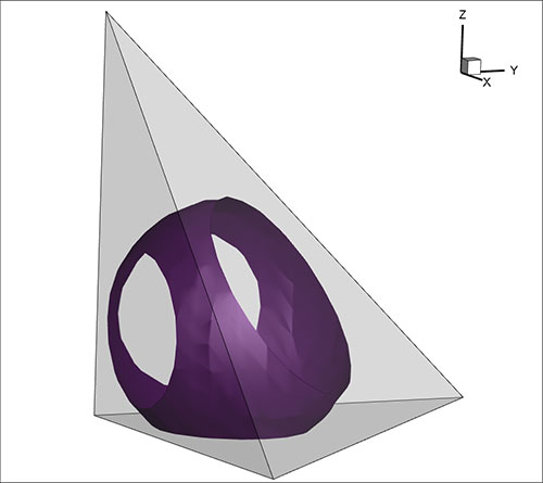
Figure 2. Isosurface in a quadratic tetrahedra.
In fact, the isosurface can be completely defined by its intersections with the edges of the tetrahedra. Since the solution varies linearly along the edges you can calculate these intersections very quickly. You can also quickly exclude edges based on the range of the nodal values at either end of the edge. If the isosurface value is greater than the maximum node value, or less than the minimum node value, no need to compute further. In this way, the vast majority of the edges can be excluded from further computation by a couple of simple floating-point compares. This, among other optimizations, make this simple technique very fast. The equivalent algorithms (marching cubes) for hexahedra is a little more complex, but the same sort of optimizations apply.
Isosurface in a quadratic Tetrahedra
No such simple isosurface algorithm exists for higher-order elements. The isosurface is not, in general, planar and it doesn’t even have to intersect the edges or surfaces of the element (see Figure 2). You can have isosurfaces that are entirely contained within an element like little islands. It demands a new and, most likely, more computationally expensive algorithm.
Other areas of visualization are also complicated by the use of higher-order elements. Surface shading, mesh plots, interpolations for streamtrace computation (and other things) all must be modified.
In my next blog, I will discuss the results of our research into higher-order finite-element isosurface algorithms. See all blogs on higher order elements.
Subscribe to Tecplot 360
Get notified when the next blog is posted!