


 MENU
MENUWhen it comes to PIV, Tecplot 360 is the real MVP.
PIV, or Particle Image Velocimetry, is a method of experimental flow visualization that uses seeding particles and some form of camera or optics to measure 2- or 3-dimensional vector fields. It can be an extremely powerful way to capture “real life” (in quotes due to the errors and assumptions inherent in any experiment!) flow physics so as not to be fully reliant on computational methods. But, just as with computational methods, the output of the experiment is a ton of numerical data – what then?
Enter Tecplot 360, which is used in conjunction with every major PIV system to visualize and analyze the recorded data. 360 has everything you might need to get the most out of your PIV data; it can handle 3D data, 2D data, XY plots, animations, text & graphical annotations, and can even compare your PIV data against CFD results for the same experiment.
3D Data
For 3D measurements, like tomographic PIV, 360 can produce high-quality movies for transient cases. In steady-state cases, 360 can create plots of amazing quality.
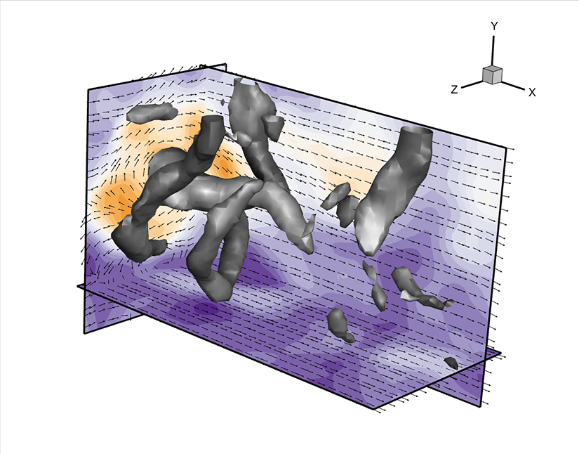
3D model plus PIV slices
TomoPIV Animation from La Vision
You can easily combine data from arbitrary sources with 360. One option is to compare PIV slices which have been measured at different heights with the corresponding 3D CAD model. The import of the CAD model is done with 360’s STL loader.
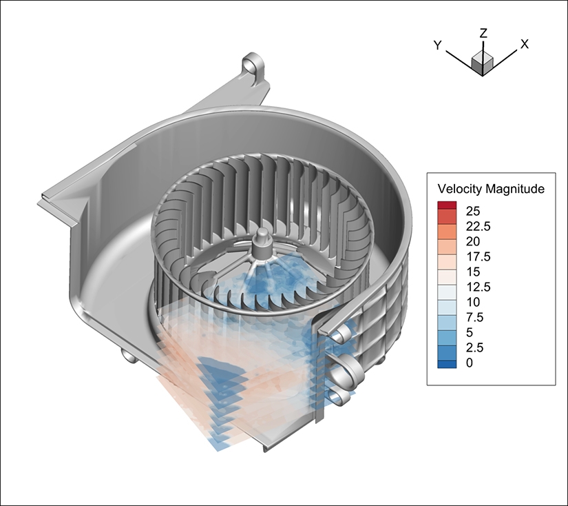
3D Model combined with PIV planes, done with Dantec Dynamics, data from Valeo
2D Data
The classic output from a PIV system is 2D measurement data.
Here again you may have transient cases that you might wish to animate. Another great feature of 360 is the extraction of point probes over time. You may wish to do a Fourier transform to understand fluctuations better. Or perhaps you will want to extract profile lines in stationary and transient cases and perform some statistical analysis (if not already given by your PIV system) such as the calculation of mean values, standard derivation, measurement of turbulent energy, etc. With 360 any of these analyses or visualization tasks are easy to perform out of the box.
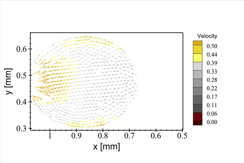
2D Droplet Visualization Vectorfield
2D flow over time around obstacle
XY Plots
XY plots are often used to create various line plots from extracted profile data. Here is an example from the 2D animation for the first timestep.
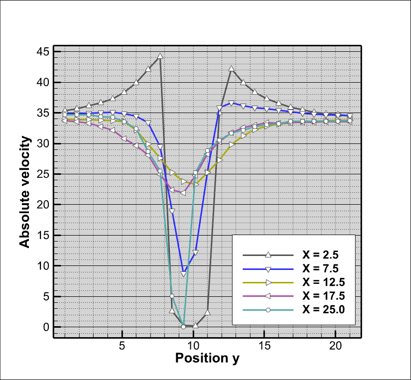
XY Profile Lines
Animations
High-quality animations from several different types of plots are easily created with 360. You also have the freedom to arrange animations over multiple frames, allowing multiple animations to play in a synchronized manner, as in the animations above.
Text or Graphical Annotations
360 allows the user to anchor text or geometric annotations (vectors, lines, circles, rectangles, …) to specific locations in your plot. This helps the audience to understand your work better by adding context to your visuals.
2D PIV Data Combined with 3D Simulation Data
Oftentimes CFD groups work closely together with PIV or other measurement groups. 360 is perfectly able to load all the different data types. You can compare the data, create difference plots, show the PIV slices in 3D together with CFD results, etc.
Suffice to say, if you have a PIV visualization or analysis task in mind the odds are good that 360 can help you accomplish it.
Tips and Tricks for PIV Post-Processing
PIV systems can produce a wide variety of data formats. Fortunately, 360 makes it simple to handle most formats, and even for more esoteric data formats there is usually a path to load your data. Briefly we’ll describe some common workflows, but if you need more help, please don’t hesitate to contact our fantastic support team (support@tecplot.com).
#1 The ideal case:
If your data is already in Tecplot format via export or data loaders (for example, via Dantec, La Vision, TSI), you won’t have to do much. You may wish to scale your data or rotate/translate it to align with your preferred reference frame. If so, read case #4 below.
#2 The 2D measurement data is ASCII, but contains only points, not the structure as an IJ-ordered matrix:
Use the General Text loader and, if needed, give the data a structure.
- Triangulation. In 2D mode, Data > 2D triangulation. This will create a triangular mesh connecting the data points.
- Linear interpolation: First, triangulate the data (this is required for linear interpolation, but not required if you use inverse-distance interpolation). Now, go to 2D mode, select Data > Create Zone > Rectangular, in order to create a IJ-ordered mesh matrix. Here you can linear interpolate, Data > Interpolate > Linear, in order to interpolate the source zone data in the triangulation to the rectangular, IJ-ordered zone.
#3 The data is transient, but time information is missing:
We have a tool which assigns time information to the zones. After loading your data, you might see that the time slider in the Plot sidebar is greyed out. In the Zone Style, you will see all timesteps as single zones. If you want to assign solution times to your data, select Data > Edit Time Strands which allows you to assign the correct timesteps.
#4 The data must be rotated, translated, or scaled:
- To scale the data, go to Data > Alter > Specify Equations and use an assignment (= “Equation”), such as x = x/1000 to convert millimeters to meters in the x-direction.
- To translate the data, go to Data > Alter > Specify Equations and use an assignment like x = x + 1.2 to translate the data 1.2 units in the positive x-axis direction.
- To rotate the data, you will use in 2D mode: Data > Alter > Axial Rotation. Be sure that you correctly assigned the vector field first (simply activate the vector layer). This will rotate the vector field accordingly.
#5 Data is loaded, but more variables must be calculated:
To compute new variables from your existing dataset, use “Specify Equations” for simple cases. Alternatively, you can calculate CFD Analyze variables with Analyze > Field Variables to select the correct vector field first, and then choose the desired computation (i.e. Analyze > Calculate Variables > Velocity Magnitude). The full spectrum of possibilities is available using 360 together with PyTecplot, which is 360’s Python API. Use the Python API to compute more complex variables, such as the standard deviation of velocity in each timestep compared to the mean velocity over time, or multidimensional Fourier transforms.
#6 You find you must perform certain tasks repeatedly:
Use either 360’s intrinsic macro language or PyTecplot to perform repeated tasks programmatically. Either of these options allows a full automation and adaption to your workflow.
Learn More and Try Tecplot 360 For Free!
Again, please feel free to ask the Support Team for help with these tasks or anything else! They are eager to help! Also, take a look at our existing tutorial videos to gain further insight into the wide range of 360’s capabilities.